Getting started

As PyCoTools only provides an alternative interface into some of COPASI’s tasks, if you are unfamiliar with COPASI, it is a good idea to become acquainted prior to proceeding. As much as possible, arguments to PyCoTools functions follow the corresponding option in the COPASI user interface.

In addition to COPASI, PyCoTools depends on tellurium which is a Python package for modelling biological systems. While tellurium and COPASI have some of the same features, generally they are complementary and productivity is enhanced by using both together.

More specifically, tellurium uses antimony strings to define a model which is then converted into SBML. PyCoTools provides the model.BuildAntimony class which is a wrapper around this tellurium feature, which creates a Copasi model and parses it into a PyCoTools model.Model.

Since antimony is described elsewhere we will focus here on using antimony to build a copasi model.

Build a model with antimony

import site, os
from pycotools3 import model

working_directory = os.path.abspath('') #create a base directory to work from
copasi_filename = os.path.join(working_directory, 'NegativeFeedbackModel.cps') #create a string to a copasi file on system
antimony_string =  '''
    model negative_feedback()
        // define compartments
        compartment cell = 1.0
        //define species
        var A in cell
        var B in cell
        //define some global parameter for use in reactions
        vAProd = 0.1
        kADeg  = 0.2
        kBProd = 0.3
        kBDeg  = 0.4
        //define initial conditions
        A      = 0
        B      = 0
        //define reactions
        AProd:  => A; cell*vAProd
        ADeg: A =>  ; cell*kADeg*A*B
        BProd:  => B; cell*kBProd*A
        BDeg: B =>  ; cell*kBDeg*B
    end
    '''
negative_feedback = model.loada(antimony_string, copasi_filename) # load the model
print(negative_feedback)
assert os.path.isfile(copasi_filename) #check that the model exists

Model(name=negative_feedback, time_unit=s, volume_unit=l, quantity_unit=mol)

Create an antmiony string from an existing model

The Copasi user interface is an excellant way of constructing a model and it is easy to convert this model into an antimony string that can be pasted into a document.

print(negative_feedback.to_antimony())

// Created by libAntimony v2.9.4
function Constant_flux__irreversible(v)
  v;
end

function Function_for_ADeg(A, B, kADeg)
  kADeg*A*B;
end

function Function_for_BProd(A, kBProd)
  kBProd*A;
end


model *negative_feedback()

  // Compartments and Species:
  compartment cell;
  species A in cell, B in cell;

  // Reactions:
  AProd:  => A; cell*Constant_flux__irreversible(vAProd);
  ADeg: A => ; cell*Function_for_ADeg(A, B, kADeg);
  BProd:  => B; cell*Function_for_BProd(A, kBProd);
  BDeg: B => ; cell*kBDeg*B;

  // Species initializations:
  A = 0;
  B = 0;

  // Compartment initializations:
  cell = 1;

  // Variable initializations:
  vAProd = 0.1;
  kADeg = 0.2;
  kBProd = 0.3;
  kBDeg = 0.4;

  // Other declarations:
  const cell, vAProd, kADeg, kBProd, kBDeg;
end

One paradigm of model development is to use antimony to ‘hard code’ perminent changes to the model and the Copasi user interface for experimental changes. The Model.open() method is useful for this paradigm as it opens the model with whatever configurations have been defined.

negative_feedback.open()

Simulate a time course

Since we have used an antimony string, we can simulate this model with either tellurium or Copasi. Simulating with tellurium uses a library called roadrunner which is described in detail elsewhere. To run a simulation with Copasi we need to configure the time course task, make the task executable (i.e. tick the check box in the top right of the time course task) and run the simulation with CopasiSE. This is all taken care of by the tasks.TimeCourse class.

from pycotools3 import tasks
time_course = tasks.TimeCourse(negative_feedback, end=100, step_size=1, intervals=100)
time_course

<pycotools3.tasks.TimeCourse at 0x1ff411e5588>

However a more convenient interface is provided by the model.simulate method, which is a wrapper around tasks.TimeCourse which additionally parses the resulting data from file and returns a pandas.DataFrame

from pycotools3 import tasks
fname = os.path.join(os.path.abspath(''), 'timcourse.txt')
sim_data = negative_feedback.simulate(0, 100, 1, report_name=fname) ##start, end, by
sim_data.head()

	A	B
Time
0	0.000000	0.000000
1	0.099932	0.013181
2	0.199023	0.046643
3	0.295526	0.093275
4	0.387233	0.147810

The results are saved in a file defined by the report_name option, which defaults to timecourse.txt in the same directory as the copasi model.

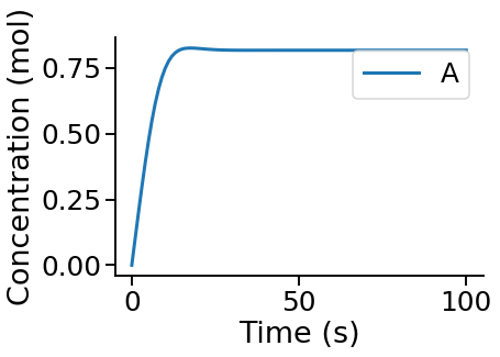
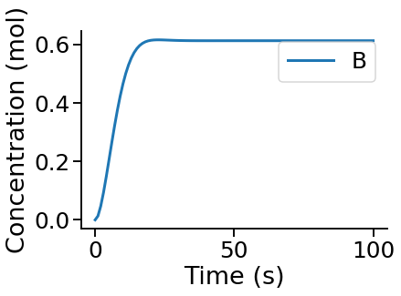
Visualise a time course

PyCoTools also provides facilities for visualising simulation output. To plot a timecourse, pass the task.TimeCourse object to the viz.PlotTimeCourse object.

from pycotools3 import viz
viz.PlotTimeCourse(time_course, savefig=True)

<pycotools3.viz.PlotTimeCourse at 0x1ff411e53c8>

More information about running time courses with PyCoTools and Copasi can be found in the time course tutorial

Run Parameter Estimation

The following configures a regular copasi parameter estimation (context='s') on all global and initial concentration parameters (parameters='gm') using the genetic algorithm

from pycotools3 import tasks, viz

with tasks.ParameterEstimation.Context(negative_feedback, fname, context='s', parameters='gm') as context:
    context.set('randomize_start_values', True)
    context.set('method', 'genetic_algorithm')
    context.set('population_size', 50)
    context.set('number_of_generations', 300)
    context.set('run_mode', True) ##defaults to False
    context.set('pe_number', 2) ## number of repeat items in scan task
    context.set('copy_number', 2) ## number of times to copy model
    config = context.get_config()

pe = tasks.ParameterEstimation(config)
data = viz.Parse(pe)
print(data)

{'NegativeFeedbackModel':           A         B       RSS     kADeg     kBDeg    kBProd    vAProd
0  0.000004  0.000321  0.000348  0.198104  0.404187  0.298985  0.099467
1  0.000397  0.000009  0.000358  0.201986  0.396722  0.296337  0.100254
2  0.002442  0.000002  0.000399  0.197253  0.403480  0.299229  0.099694
3  0.110722  0.004461  0.002555  0.198449  0.402032  0.297208  0.097885}

pycotools3 supports the configuration of:

• multiple models at once
• multiple parameter estimation repeats at once
• profile likelihoods
• cross validations

Also you can checkout the parameter estimation tutorial.